Josef “Jeff” Sipek

After several years of having a desktop at home that’s been unplugged and unused I decided that it was time to make a home server to do some of my development on and just to keep files stored safely and redundantly. This was in August 2011. A lot has happened since then. First of all, I rebuilt the OpenIndiana (an Illumos-based distribution) setup with SmartOS (another Illumos-based distribution). Since I wrote most of this a long time ago, some of the information below is obsolete. I am sharing it anyway since others may find it useful. Toward the end of the post, I’ll go over SmartOS rebuild. As you may have guessed, the hostname for this box ended up being  Isis.

First of all, I should list my goals.

storage box

The obvious mix for digital photos, source code repositories, assorted documents, and email backup is easy enough to store. It however becomes a nightmare if you need to keep track where they are (i.e., which of the two external disks, public server (Odin), laptop drives, desktop drives they are on). Since none of them are explicitly public, it makes sense to keep them near home instead on my public server that’s in a data-center with a fairly slow uplink (1 Mbit/s burstable to 10 Mbits/s, billed at 95th percentile).

dev box

I have a fast enough laptop (Thinkpad T520), but a beefier system that I can let compile large amounts of code is always nice. It will also let me run several virtual machines and zones comfortably — for development, system administration experiments, and other fun stuff.

router

I have an old Linksys WRT54G (rev. 3) that has served me well for the years. Sadly, it is getting a bit in my way — IPv6 tunneling over IPv4 is difficult, the 100 Mbit/s switch makes it harder to transfer files between computers, etc. If I am making a server that will be always on, it should handle effortlessly NAT’ing my Comcast internet connection. Having a full-fledged server doing the routing will also let me do better traffic shaping & filtering to make the connection feel better.

Now that you know what sort of goals I have, let’s take a closer look at the requirments for the hardware.

1. reliable
2. friendly to OpenIndiana and ZFS
3. low-power
4. fast
5. virtualization assists (to support run virtual machines at reasonable speed)
6. cheap
7. quiet
8. spacious (storage-wise)

While each one of them is pretty easy to accomplish, their combination is much harder to achieve. Also note that it is ordered from most to least important. As you will see, reliability dictated many of my choices.

The Shopping List

CPU

Intel Xeon E3-1230 Sandy Bridge 3.2GHz LGA 1155 80W Quad-Core Server Processor BX80623E31230

RAM (4)

Kingston ValueRAM 4GB 240-Pin DDR3 SDRAM DDR3 1333 ECC Unbuffered Server Memory Model KVR1333D3E9S/4G

Motherboard

SUPERMICRO MBD-X9SCL-O LGA 1155 Intel C202 Micro ATX Intel Xeon E3 Server Motherboard

Case

SUPERMICRO CSE-743T-500B Black Pedestal Server Case

Data Drives (3)

Seagate Barracuda Green ST2000DL003 2TB 5900 RPM SATA 6.0Gb/s 3.5"

System Drives (2)

Western Digital WD1600BEVT 160 GB 5400RPM SATA 8 MB 2.5-Inch Notebook Hard Drive

Additional NIC

Intel EXPI9301CT 10/100/1000Mbps PCI-Express Desktop Adapter Gigabit CT

To measure the power utilization, I got a P3 International P4400 Kill A Watt Electricity Usage Monitor. All my power usage numbers are based on watching the digital display.

Intel vs. AMD

I’ve read Constantin’s OpenSolaris ZFS Home Server Reference Design and I couldn’t help but agree that ECC should be a standard feature on all processors. Constantin pointed out that many more AMD processors support ECC and that as long as you got a motherboard that supported it as well you are set. I started looking around at AMD processors but my search was derailed by Joyent’s announcement that they ported KVM to Illumos — the core of OpenIndiana including the kernel. Unfortunately for AMD, this port supports only Intel CPUs. I switched gears and started looking at Intel CPUs.

In a way I wish I had a better reason for choosing Intel over AMD but that’s the truth. I didn’t want to wait for AMD’s processors to be supported by the KVM port.

So, why did I get a 3.2GHz Xeon (E3-1230)? I actually started by looking for motherboards. At first, I looked at desktop (read: cheap) motherboards. Sadly, none of the Intel-based boards I’ve seen supported ECC memory. Looking at server-class boards made the search for ECC support trivial. I was surprised to find a Supermicro motherboard (MBD-X9SCL-O) for $160. It supports up to 32 GB of ECC RAM (4x 8 GB DIMMs). Rather cheap, ECC memory, dual gigabit LAN (even though one of the LAN ports uses the Intel 82579 which was unsupported by OpenIndiana at the time), 6 SATA II ports — a nice board by any standard. This motherboard uses the LGA 1155 socket. That more or less means that I was “stuck” with getting a Sandy Bridge processor. :-D The E3-1230 is one of the slower E3 series processors, but it is still very fast compared to most of the other processors in the same price range. Additionally, it’s “only” 80 Watt chip compared to many 95 or even 130 Watt chips from the previous series.

There you have it. The processor was more or less determined by the motherboard choice. Well, that’s being rather unfair. It just ended up being a good combination of processor and motherboard — a cheap server board and near-bottom-of-the-line processor that happens to be really sweet.

Now that I had a processor and a motherboard picked out, it was time to get RAM. In the past, I’ve had good luck with Kingston, and since it happened to be the cheapest ECC 4 GB DIMMs on NewEgg, I got 4 — for a grand total of 16 GB.

Case

I will let you know a secret. I love hotswap drive bays. They just make your life easier — from being able to lift a case up high to put it on a shelf without having to lift all those heavy drives at the same time, to quickly replacing a dead drive without taking the whole system down.

I like my public server’s case (Supermicro CSE-743T-645B) but the 645 Watt power supply is really an overkill for my needs. The four 5000 RPM fans on the midplane are pretty loud when they go full speed. I looked around, and I found a 500 Watt (80%+ efficiency) variant of the case (CSE-743-500B). Still a beefy power supply but closer to what one sees in high end desktops. With this case, I get eight 3.5" hot-swap bays, and three 5.25" external (non-hotswap) bays. This case shouldn’t be a limiting factor in any way.

I intended to move my DVD+RW drive from my desktop but that didn’t work out as well as I hoped.

Storage

At the time I was constructing Isis, I was experimenting with  ZFS on OpenIndiana. I was more than impressed, and I wanted it to manage the storage on my home sever. ZFS is more than just a filesystem, it is also a volume manager. In other words, you can give it multiple disks and tell it to put your data on them in several different ways that closely resemble RAID levels. It can stripe, mirror, or calculate one to three parities. Wikipedia has a nice article outlining ZFS’s features. Anyway, I strongly support ZFS’s attitude toward losing data — do everything to prevent it in the first place.

Hard drives are very interesting devices. Their reliability varies with so many variables (e.g., manufacturing defects, firmware bugs). In general, manufacturers give you fairly meaningless looking, yet impressive sounding numbers about their drives reliability. Richard Elling made a great blog post where he analyzed ZFS RAID space versus Mean-Time-To-Data-Loss, or MTTDL for short. (Later, he analyzed a different MTTDL model.)

The short version of the story is nicely summed up by this graph (taken from Richard’s blog):

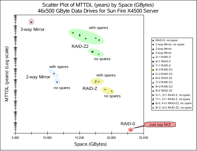
While this scatter plot is for a specific model of a high-end server, it applies to storage in general. I like how the various types of redundancy clump up.

Anyway, how much do I care about my files? Most of my code lives in distributed version control systems, so losing one machine wouldn’t be a problem for those. The other files would be a bigger problem. While it wouldn’t be a complete end of the world if I lost all my photos, I’d rather not lose them. This goes back to the requirements list — I prefer reliable over spacious. That’s why I went with 3-way mirror of 2 TB Seagate Barracuda Green drives. It gets me only 2 TB of usable space, but at the same time I should be able to keep my files forever. These are the data drives. I also got two 2.5" 160 GB Western Digital laptop drives to hold the system files — mirrored of course.

Around the same time I was discovering that the only sane way to keep your files was mirroring, I stumbled across Constantin’s RAID Greed post. He basically says the same thing — use 3-way mirror and your files will be happy.

Now, you might be asking… 2 TB, that’s not a lot of space. What if you out grow it? My answer is simple: ZFS handles that for me. I can easily buy three more drives, plug them in and add them as a second 3-way mirror and ZFS will happily stripe across the two mirrors. I considered buying 6 disks right away, but realized that it’ll probably be at least 6-9 months before I’ll have more than 2 TB of data. So, if I postpone the purchase of the 3 additional drives, I can save money. It turns out that a year and a half later, I’m still below 70% of the 2 TB.

Miscellaneous

I knew that one of the on-board LAN ports was not yet supported by Illumos, and so I threw a PCI-e Gigabit ethernet card into the shopping cart. I went with an Intel gigabit card. Illumos has since gained support for 82579-based NICs, but I’m lazy and so I’m still using the PCI-e NIC.

Base System

As the ordered components started showing up, I started assembling them. Thankfully, the CPU, RAM, motherboard, and case showed up at the same time preventing me from going crazy. The CPU came with a stock Intel heatsink.

The system started up fine. I went into the BIOS and did the usual new-system tweaking — make sure SATA ports are in AHCI mode, stagger the disk spinup to prevent unnecessary load peaks at boot, change the boot order to skip PXE, etc. While roaming around the menu options, I discovered that the motherboard can boot from iSCSI. Pretty neat, but useless for me on this system.

The BIOS has a menu screen that displays the fan speeds and the system and processor temperatures. With the fan on the heatsink and only one midplane fan connected the system ran at about 1°C higher than room temperature and the CPU was about 7°C higher than room temperature.

OS Installation

Anyway, it was time to install OpenIndiana. I put my desktop’s DVD+RW in the case and then realized that the motherboard doesn’t have any IDE ports! Oh well, time to use a USB flash drive instead. At this point, I had only the 2 system drives. I connected one to the first SATA port, put a 151 development snapshot (text installer) on my only USB flash drive. The installer booted just fine. Installation was uneventful. The one potentially out of the ordinary thing I did was to not configure any networking. Instead, I set it up manually after the first boot, but more about that later.

With OI installed on one disk, it was time to set up the rpool mirror. I used Constantin’s Mirroring Your ZFS Root Pool as the general guide even though it is pretty straight forward — duplicate the partition (and slice) scheme on the second disk, add the new slice to the root pool, and then install grub on it. Everything worked out nicely.

# zpool status rpool
  pool: rpool
 state: ONLINE
  scan: scrub repaired 0 in 0h5m with 0 errors on Sun Sep 18 14:15:24 2011
config:

        NAME          STATE     READ WRITE CKSUM
        rpool         ONLINE       0     0     0
          mirror-0    ONLINE       0     0     0
            c2t0d0s0  ONLINE       0     0     0
            c2t1d0s0  ONLINE       0     0     0

errors: No known data errors

Networking

Since I wanted this box to act as a router, the network setup was a bit more…complicated (and quite possibly over-engineered). This is why I elected to do all the network setup by hand later than having to “fix” whatever damage the installer did. :)

I powered it off, put in the extra ethernet card I got, and powered it back on. To my surprise, the new device didn’t show up in dladm. I remembered that I should trigger the device reconfiguration. A short touch /reconfigure && reboot later, dladm listed two physical NICs.

As you can see, I decided that the routing should be done in a zone. This way, all the routing settings are nicely contained in a single place that does nothing else.

Setting up the virtual interfaces was pretty easy thanks to dladm. Setting the static IP on the global zone was equally trivial.

# dladm create-vlan -l e1000g0 -v 11 vlan11
# dladm create-vnic -l e1000g0 vlan0
# dladm create-vnic -l e1000g0 internal0
# dladm create-vnic -l e1000g1 isp0
# dladm create-etherstub zoneswitch0
# dladm create-vnic -l zoneswitch0 zone_router0

# ipadm create-if internal0
# ipadm create-addr -T static -a local=10.0.0.2/24 internal/v4

You might be wondering about the vlan11 interface that’s on a separate  VLAN. The idea was to have my WRT54G continue serving as a wifi access point, but have all the traffic end up on VLAN #11. The router zone would then get to decide whether the user is worthy of LAN or Internet access. I never finished poking around the WRT54G to figure out how to have it dump everything on a VLAN #11 instead of the default #0.

Router zone

OpenSolaris (and therefore all Illumos derivatives) has a wonderful feature called  zones. It is essentially a super-lightweight virtualization mechanism. While talking to a couple of people on IRC, I decided that I, like them, would use a dedicated zone as a router.

Just before I set up the router zone, the storage disks arrived. The router zone ended up being stored on this array. See the storage section below for details about this storage pool.

After installing the zone via zonecfg and zoneadm, it was time to set up the routing and firewalling. First, install the ipfilter package (pkg install pkg:/network/ipfilter). Now, it is time to configure the NAT and filter rules.

NAT is easy to set up. Just plop a couple of lines into /etc/ipf/ipnat.conf:

map isp0 10.0.0.0/24 -> 0/32 proxy port ftp ftp/tcp
map isp0 10.0.0.0/24 -> 0/32 portmap tcp/udp auto
map isp0 10.0.0.0/24 -> 0/32

map isp0 10.11.0.0/24 -> 0/32 proxy port ftp ftp/tcp
map isp0 10.11.0.0/24 -> 0/32 portmap tcp/udp auto
map isp0 10.11.0.0/24 -> 0/32

map isp0 10.1.0.0/24 -> 0/32 proxy port ftp ftp/tcp
map isp0 10.1.0.0/24 -> 0/32 portmap tcp/udp auto
map isp0 10.1.0.0/24 -> 0/32

IPFilter is a bit trickier to set up. The rules need to handle more cases. In general, I tried to be a bit paranoid about the rules. For example, I drop all traffic for IP addresses that don’t belong on that interface (I should never see 10.0.0.0/24 addresses on my ISP interface). The only snag was in the defaults for the ipfilter  SMF service. By default, it expects you to put your rules into SMF properties. I wanted to use the more old-school approach of using a config file. Thankfully, I quickly found a blog post which hepled me with it.

Storage, part 2

As the list of components implies, I wanted to make two arrays. I already mentioned the rpool mirror. Once the three 2 TB disks arrived, I hooked them up and created a 3-way mirror (zpool create storage mirror c2t3d0 c2t4d0 c2t5d0).

# zpool status storage
  pool: storage
 state: ONLINE
  scan: scrub repaired 0 in 0h0m with 0 errors on Sun Sep 18 14:10:22 2011
config:

        NAME        STATE     READ WRITE CKSUM
        storage     ONLINE       0     0     0
          mirror-0  ONLINE       0     0     0
            c2t3d0  ONLINE       0     0     0
            c2t4d0  ONLINE       0     0     0
            c2t5d0  ONLINE       0     0     0

errors: No known data errors

Deduplication & Compression

I suspected that there would be enough files that would be stored several times — system binaries for zones, clones of source trees, etc. ZFS has built-in online  deduplication. This stores each unique block only once. It’s easy enough to turn on: zfs set dedup=on storage.

Additionally, ZFS has transparent data (and metadata) compression featuring  LZJB and gzip algorithms.

I enabled dedup and kept compression off. Dedup did take care of the duplicate binaries between all the zones. It even took care of duplicates in my photo stash. (At some point, I managed to end up with several diverged copies of my photo stash. One of the first things I did with Isis, was to dump all of them in the same place and start sorting them. Adobe Lightroom helped here quite a bit.)

After a while, I came to the realization that for most workloads I run, dedup was wasteful and I would be better off disabling dedup and enabling light compression (i.e., LZJB).

$HOME

The installer puts the non-privileged user’s home directory onto the root pool. I did not want to keep it there since I now had the storage pool. After a bit of thought, I decided to zfs create storage/home and then transfer over the current home directory. I could have used cp(1) or rsync(1), but I thought it would be more fun (and a learning experience) to use zfs send and zfs recv. It went something like this:

# zfs snapshot rpool/export/home/jeffpc@snap
# zfs send rpool/export/home/jeffpc@snap | zfs recv storage/home/jeffpc

In theory, any modifications to my home directory after the snapshot got lost, but since I was just ssh’d in there wasn’t much that changed. (I am ok with losing the last update to .bash_history this one time.) The last thing that needed changing is /etc/auto_home — which tells the automounter where my $HOME really is. This is the resulting file after the change (without the copyright comment):

jeffpc	localhost:/storage/home/&
+auto_home

For good measure, I rebooted to make sure things would come up properly — they did.

Since the server is not intended just for me, I created the other user account with a home directory in storage/home/holly.

Zones

I intend to use zones extensively. To keep their files out of the way, I decided on storage/zones/$ZONE_NAME. I’ll talk more about the zones I set up later in the Zones section.

SMB

Local storage is great, but there is only so much you can do with it. Sooner or later, you will want to access it from a different computer. There are many different ways to “export” your data, but as one might expert, they all have their benefits and drawbacks. ZFS makes it really easy to export data via NFS and SMB. After a lot of thought, I decided that SMB would work a bit better. The major benefit of SMB over NFS is that it Just Works™ on all the major operating systems. That’s not to say that NFS does not work, but rather that it needs a bit more…convincing at times. This is especially true on Windows.

I followed the documentation for enabling SMB on Solaris 11. Yes, I know, OpenIndiana isn’t Solaris 11, but this aspect was the same. This ended with me enabling sharing of several datasets like this:

# zfs set sharesmb=name=photos storage/photos

ACLs

The home directory shares are all done. The photos share, however, needs a bit more work. Specifically, it should be fully accessible to the users that are supposed to have access (i.e., jeffpc & holly). The easiest way I can find is to use ZFS ACLs.

First, I set the aclmode to passthrough (zfs set aclmode=passthough storage). This will prevent a chmod(1) on a file or directory from blowing away all the ACEs (Access Control Entries?). Then on the share directory, I added two ACL entries that allow everything.

# /usr/bin/ls -dV /share/photos
drwxr-xr-x   2 jeffpc   root           4 Sep 23 09:12 /share/photos
                 owner@:rwxp--aARWcCos:-------:allow
                 group@:r-x---a-R-c--s:-------:allow
              everyone@:r-x---a-R-c--s:-------:allow
# /usr/bin/chmod A+user:jeffpc:rwxpdDaARWcCos:fd:allow /share/photos
# /usr/bin/chmod A+user:holly:rwxpdDaARWcCos:fd:allow /share/photos
# /usr/bin/chmod A2- /share/photos # get rid of user
# /usr/bin/chmod A2- /share/photos # get rid of group
# /usr/bin/chmod A2- /share/photos # get rid of everyone
# /usr/bin/ls -dV /share/photos
drwx------+  2 jeffpc   root           4 Sep 23 09:12 /share/photos
            user:jeffpc:rwxpdDaARWcCos:fd-----:allow
             user:holly:rwxpdDaARWcCos:fd-----:allow

The first two chmod commands prepend two ACEs. The next three remove ACE number 2 (the third entry). Since the directory started of with three ACEs (representing the standard Unix permissions), the second set of chmods removes those, leaving only the two user ACEs behind.

Clients

That was easy! In case you are wondering, the Solaris/Illumos SMB service does not allow guest access. You must login to use any of the shares.

Anyway, here’s the end result:

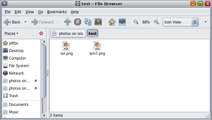
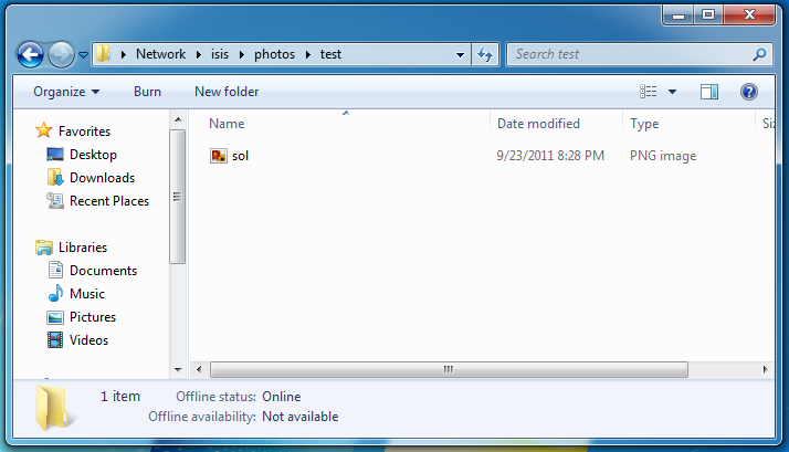
Pretty neat, eh?

Zones

Aside from the router zone, there were a number of other zones. Most of them were for Illumos and OpenIndiana development.

I don’t remember much of the details since this predates the SmartOS conversion.

Power

When I first measured the system, it was drawing about 40-45 Watts while idle. Now, I have Isis along with the WRT54G and a gigabit switch on a UPS that tells me that I’m using about 60 Watts when idle. The load can spike up quite a bit if I put load on the 4 Xeon cores and give the disks something to do. (Afterall, it is an 80 Watt CPU!) While this is by no means super low-power, it is low enough and at the same time I have the capability to actually get work done instead of waiting for hours for something to compile.

SmartOS

As I already mentioned, I ended up rebuilding the system with SmartOS. SmartOS is not a general purpose distro. Rather, it strives to be a hypervisor with utilities that make guest management trivial. Guests can either be zones, or KVM-powered virtual machines. Here are the major changes from the OpenIndiana setup.

Storage — pools

SmartOS is one of those distros you do not install. It always netboots, boots from a USB stick or a CD. As a result, you do not need a system drive. This immediately obsoleted the two laptop drives. Conveniently, around the same time, Holly’s laptop suffered from a disk failure so Isis got to donate one of the unused 2.5" system disks.

SmartOS calls its data pool “zones”, which took a little bit of getting used to. There’s a way to import other pools, but wanted to keep the settings as vanilla as possible.

At some point, I threw in a Intel 160 GB SSD to use for L2ARC and  ZIL.

Here’s what the pool looks like:

# zpool status
  pool: zones
 state: ONLINE
status: Some supported features are not enabled on the pool. The pool can
        still be used, but some features are unavailable.
action: Enable all features using 'zpool upgrade'. Once this is done,
        the pool may no longer be accessible by software that does not support
        the features. See zpool-features(5) for details.
  scan: scrub repaired 0 in 2h59m with 0 errors on Sun Jan 13 08:37:37 2013
config:

        NAME        STATE     READ WRITE CKSUM
        zones       ONLINE       0     0     0
          mirror-0  ONLINE       0     0     0
            c1t5d0  ONLINE       0     0     0
            c1t4d0  ONLINE       0     0     0
            c1t3d0  ONLINE       0     0     0
        logs
          c1t1d0s0  ONLINE       0     0     0
        cache
          c1t1d0s1  ONLINE       0     0     0

errors: No known data errors

In case you are wondering about the features related status message, I created the zones pool way back when Illumos (and therefore SmartOS) had only two ZFS features. Since then, Illumos added one and Joyent added one to SmartOS.

# zpool get all zones | /usr/xpg4/bin/grep -E '(PROP|feature)'
NAME   PROPERTY                   VALUE                      SOURCE
zones  feature@async_destroy      enabled                    local
zones  feature@empty_bpobj        active                     local
zones  feature@lz4_compress       disabled                   local
zones  feature@filesystem_limits  disabled                   local

I haven’t experimented with either enough to enable it on a production system I rely on so much.

Storage — deduplication & compression

The rebuild gave me a chance to start with a clean slate. Specifically, it gave me a chance to get rid off the dedup table. (The dedup table, DDT, is built as writes happen to the filesystem with dedup enabled.) Data deduplication relies on some form of data structure (the most trivial one is a hash table) that maps the hash of the data to the data. In ZFS, the DDT maps the  SHA-256 of the block to the block address.

The reason I stopped using dedup on my systems was pretty straight forward (and not specific to ZFS). Every entry in the DDT has an overhead. So, ideally, every entry in the DDT is referenced at least twice. If a block is referenced only once, then one would be better off without the block taking up an entry in the DDT. Additionally, every time a reference is taken or released, the DDT needs to be updated. This causes very nasty random I/O under which spinning disks want to weep. It turns out, that a “normal” user will have mostly unique data rendering deduplication impractical.

That’s why I stopped using dedup. Instead, I became convinced that most of the time light compression is the way to go. Lightly compressing the data will result in I/O bandwidth savings as well as capacity savings with little overhead given today’s processor speeds versus I/O latencies. Since I haven’t had time to experiment with the recently integrated LZ4, I still use LZJB.

A week ago (June 15), I went on my first solo cross country flight. The plan was to fly KARB → KMBS → KAMN → KARB. In case you don’t happen to have the Detroit sectional chart in front of you, this might help you visualize the scope of the flight.

Here’s the ground track (as recorded by the G1000) along with red dots for each of my checkpoints and a pink line connecting them. (Sadly, there’s no convenient zoom level that covers the entire track without excessive waste.)

As you can see, I didn’t quite overfly all the checkpoints. In my defense, the forecast winds were about 40 degrees off from reality during the first half of the flight. :)

Let’s examine each leg separately.

KARB → KMBS

My checkpoint by I-69 (southwest of Flint) was supposed to be a I-69 and Pontiac VORTAC (PSI) radial 311 intersection. However when I called up the FSS briefer, I found out that it was out of service. Thankfully, Salem VORTAC (SVM) is very close so I just used its radial 339 instead. Next time I’m using a VOR for any part of my planning, I’m going to check for any NOTAMs before I make it part of my plan — redoing portions of the plan is tedious and not fun.

On the way to Saginaw, I was planning to go at 3500. (Yes, I know, it is a westerly direction and the rule (FAR 91.159) says even thousand + 500, but the clouds were not high enough to fly at 4500 and the rule only applies 3000 AGL and above — the ground around these parts is 700-1000 feet MSL.)

Right when I entered the downwind for runway 23, the tower cleared me to land. My clearance was quickly followed by the tower instructing a commuter jet to hold short of 23 because of landing traffic — me! Somehow, it is very satisfying to see a real plane (CRJ-200) have to wait for little ol’ me to land. (FlightAware tells me that it was FLG3903 flight to KDTW.)

While I was on taxiway C, they got cleared to take off. I couldn’t help it but to snap a photo.

It was a pretty slow day for Saginaw. The whole time I was on the radio with Saginaw approach, I got to hear maybe 5 planes total. The tower was even less busy. There were no planes around except for me and the commuter jet.

KMBS → KAMN

This leg of the flight was the hardest. First of all, it was only 29 nm. This equated to about 25 minutes of flying. The first four-ish and the last five-ish were spent climbing and descending, so really there was about 15 minutes of cruising. Not much time to begin with. I flew this leg by following the MBS VOR radial 248. My one and only checkpoint on this leg was mid way — the beginning of a wind turbine farm. It took about 2 minutes longer to get there than planned, but the wind turbines were easy to see from distance so no problems there.

Following the VOR wasn’t difficult, but you can see in the ground track that I was meandering across it. As expected, it got easier the farther away from the station I got. Here’s the plot of the CDI deflection for this leg. The CSV file says that the units are “fsd” — I have no idea what that means.

I can’t really draw any conclusions because…well, I don’t know what the graph is telling me. Sure, it seems to get closer and closer to zero (which I assume is a good thing), but I can’t honestly say that I understand what the graph is saying.

The most difficult part was trying to stay at 2500 feet. For whatever reason, it felt like I was flying in sizable thermals. Since there were no thunderstorms in the area, I flew on fighting the updrafts. That was the difficult part. I suspect the wind turbines were built there because the area is windy.

KAMN is a decent size airport. Two plenty long runways for a 172 even on a hot day (5004x75 feet and 3197x75 feet). I didn’t stop by the FBO, so I have no idea how they are. I did not notice anyone else around during the couple of minutes I spent on the ground taxiing and getting ready for the next leg. Maybe it was just the overcast that made people stay indoors. Oh well. It is a nice airport, and I wouldn’t mind stopping there in the future if the need arose.

KAMN → KARB

Flying back to Ann Arbor was the easy part of the trip. The air calmed down enough that once trimmed, the plane more or less stayed at 3500 feet.

It apparently was a slow day for Lansing approach as well, as I got to hear a controller chatting with a pilot of a skydiving plane about how fast the skydivers fell to the ground. Sadly, I didn’t get to hear the end of the conversation since the controller told me to contact Detroit approach.

As far as the ground track is concerned, you can see two places where I stopped flying current heading and instead flew toward the next checkpoint visually. The first instance is a few miles north of KOZW. I spotted the airport, and since I knew I was supposed to overfly it, I turned to it and flew right over it. The second instance is by Whitmore Lake — there I looked into the distance and saw Ann Arbor. Knowing that the airport is on the south side, I just headed right toward it ignoring the planned heading. As I mentioned before in both cases, the planned course was slightly off because the winds weren’t quite like the forecast said they would be.

You can’t tell from the rather low resolution of the map, but I got to fly right over the  Michigan stadium. Sadly, I was a bit too busy flying the plane to take a photo of the field below me.

Next

With one solo cross country out of the way, I’m still trying to figure out where I want to go next. Currently, I am considering one of these flights (in no particular order):

Today I came across a blog post about Running PostgreSQL on Compression-enabled ZFS. I found the article because (1) I am a fan of  ZFS, and (2) transparent storage compression interests me. (Maybe I’ll talk about the later in the future.)

Whoever ran the benchmark decided to compare ZFS with  lzjb, ZFS with gzip, against ext3. Their analysis states that ZFS-gzip is faster than ZFS-lzjb, which is faster than ext3. They admit that the benchmark is I/O bound. Then they state that compression effectively speeds up the disk I/O by making every byte transfered contain more information. The analysis goes down the drain right after that.

While doing background research for this blog post we also got a chance to investigate some of the other features besides compression that differentiate ZFS from older file system architectures like ext3. One of the biggest differences is ZFS’s approach to scheduling disk IOs which employs explicit IO priorities, IOP reordering, and deadline scheduling in order to avoid flooding the request queues of disk controllers with pending requests.

Anyone who’s benchmarked a system should have a red flag going off after reading those sentences. My reaction was something along the lines: “What?! You know that there are at least three major differences between ZFS and ext3 in addition to compression and you still try to draw conclusions about compression effectiveness by comparing ZFS with compression against ext3?!”

All they had to do to make their analysis so much more interesting and keep me quiet was to include another set of numbers — ZFS without compression. That way, one can compare ext3 with ZFS-uncompressed to see how much difference the radically different filesystem design makes. Then one could compare ZFS-uncompressed with the lzjb and gzip data to see if compression helps. Based on the data presented, we have no idea if compression helps — we just know that compression and ZFS outperform ext3. What if ZFS without compression is 5x faster than ext3? Then using gzip (~4x faster than ext3) is actually not the fastest.

To be fair, knowing how modern disk drives behave, chances are that compressed ZFS is faster than uncompressed ZFS. Since CPU cycles are so plentiful these days, all my systems have lzjb compression enabled everywhere. I do this mostly to conserve space, but also in hopes of transferring less data to disk. Yes, this is exactly what their benchmark attempts to show. (I haven’t had a chance to experiment with the new-ish lz4 compression algorithm in ZFS.) My point here is solely about benchmark analysis and unfounded (or at least unstated) assumptions found in just about every benchmark out there.

It would seem that my two recent posts are getting noticed. On one of them, someone asked for the EGT R code I used.

After I get the CSV file of the SD card, I first clean it up. Currently, I just do it manually using Vim, but in the future I will probably script it. It turns out that Garmin decided to put a header of sorts at the beginning of each CSV. The header includes version and part numbers. I delete it. The next line appears to have units for each of the columns. I delete it as well. The remainder of the file is an almost normal CSV. I say almost normal, because there’s an inordinate number of spaces around the values and commas. I use the power of Vim to remove all the spaces in the whole file by using :%s/ //g. Then I save and quit.

Now that I have a pretty standard looking CSV, I let R do its thing.

> data <- read.csv("munged.csv")
> names(data)
 [1] "LclDate"   "LclTime"   "UTCOfst"   "AtvWpt"    "Latitude"  "Longitude"
 [7] "AltB"      "BaroA"     "AltMSL"    "OAT"       "IAS"       "GndSpd"   
[13] "VSpd"      "Pitch"     "Roll"      "LatAc"     "NormAc"    "HDG"      
[19] "TRK"       "volt1"     "volt2"     "amp1"      "amp2"      "FQtyL"    
[25] "FQtyR"     "E1FFlow"   "E1OilT"    "E1OilP"    "E1RPM"     "E1CHT1"   
[31] "E1CHT2"    "E1CHT3"    "E1CHT4"    "E1EGT1"    "E1EGT2"    "E1EGT3"   
[37] "E1EGT4"    "AltGPS"    "TAS"       "HSIS"      "CRS"       "NAV1"     
[43] "NAV2"      "COM1"      "COM2"      "HCDI"      "VCDI"      "WndSpd"   
[49] "WndDr"     "WptDst"    "WptBrg"    "MagVar"    "AfcsOn"    "RollM"    
[55] "PitchM"    "RollC"     "PichC"     "VSpdG"     "GPSfix"    "HAL"      
[61] "VAL"       "HPLwas"    "HPLfd"     "VPLwas"   

As you can see, there are lots of columns. Before doing any plotting, I like to convert the LclDate, LclTime, and UTCOfst columns into a single Time column. I also get rid of the three individual columns.

> data$Time <- as.POSIXct(paste(data$LclDate, data$LclTime, data$UTCOfst))
> data$LclDate <- NULL
> data$LclTime <- NULL
> data$UTCOfst <- NULL

Now, let’s focus on the EGT values — E1EGT1 through E1EGT4. E1 refers to the first engine (the 172 has only one), I suspect that a G1000 on a twin would have E1 and E2 values. I use the ggplot2 R package to do my graphing. I could pick colors for each of the four EGT lines, but I’m way too lazy and the color selection would not look anywhere near as nice as it should. (Note, if you have only two values to plot, R will use a red-ish and a blue-ish/green-ish color for the lines. Not exactly the smartest selection if your audience may include someone color-blind.) So, instead I let R do the hard work for me. First, I make a new data.frame that contains the time and the EGT values.

> tmp <- data.frame(Time=data$Time, C1=data$E1EGT1, C2=data$E1EGT2,
                    C3=data$E1EGT3, C4=data$E1EGT4)
> head(tmp)
                 Time      C1      C2      C3      C4
1 2013-06-01 14:24:54 1029.81 1016.49 1019.08 1098.67
2 2013-06-01 14:24:54 1029.81 1016.49 1019.08 1098.67
3 2013-06-01 14:24:55 1030.94 1017.57 1019.88 1095.38
4 2013-06-01 14:24:56 1031.92 1019.05 1022.81 1095.84
5 2013-06-01 14:24:57 1033.16 1020.23 1022.82 1092.38
6 2013-06-01 14:24:58 1034.54 1022.33 1023.72 1085.82

Then I use the reshape2 package to reorganize the data.

> library(reshape2)
> tmp <- melt(tmp, "Time", variable.name="Cylinder")
> head(tmp)
                 Time Cylinder   value
1 2013-06-01 14:24:54       C1 1029.81
2 2013-06-01 14:24:54       C1 1029.81
3 2013-06-01 14:24:55       C1 1030.94
4 2013-06-01 14:24:56       C1 1031.92
5 2013-06-01 14:24:57       C1 1033.16
6 2013-06-01 14:24:58       C1 1034.54

The melt function takes a data.frame along with a name of a column (I specified “Time”), and reshapes the data.frame. For each row, in the original data.frame, it takes all the columns not specified (e.g., not Time), and produces a row for each with a variable name being the column name and the value being that column’s value in the original row. Here’s a small example:

> df <- data.frame(x=c(1,2,3),y=c(4,5,6),z=c(7,8,9))
> df
  x y z
1 1 4 7
2 2 5 8
3 3 6 9
> melt(df, "x")
  x variable value
1 1        y     4
2 2        y     5
3 3        y     6
4 1        z     7
5 2        z     8
6 3        z     9

As you can see, the x values got duplicated since there were two other columns. Anyway, the one difference in my call to melt is the variable.name argument. I don’t want my variable name column to be called “variable” — I want it to be called “Cylinder.”

At this point, the data is ready to be plotted.

> library(ggplot2)
> p <- ggplot(tmp)
> p <- p + ggtitle("Exhaust Gas Temperature")
> p <- p + ylab(expression(Temperature~(degree*F)))
> p <- p + geom_line(aes(x=Time, y=value, color=Cylinder))
> print(p)

That’s all there is to it! There may be a better way to do it, but this works for me. I use the same approach to plot the different altitude numbers, the speeds (TAS, IAS, GS), CHT, and fuel quantity.

You can download an R script with the above code here.

About a week ago, I talked about G1000 data logging. In that post, I mentioned that cross-country flying would be interesting to visualize. Well, on Friday I got to do a mock pre-solo cross country phase check. I had the G1000 logging the trip.

First of all, the plan was to fly from KARB to KFPK. It’s a 51nm trip. I had four checkpoints. For the purposes of plotting the flight, I had to convert the pencil marks on my sectional chart to latitude and longitude.

> xc_checkpoints
          Name Latitude Longitude
1      Chelsea 42.31667 -84.01667
2       Munith 42.37500 -84.20833
3       Leslie 42.45000 -84.43333
4 Eaton Rapids 42.51667 -84.65833

First of all, let’s take a look at the ground track.

In addition to just the ground track, I plotted here the first three checkpoints in red, the location of the plane every 5 minutes in blue (excluding all the data points near the airport), and some other places of interest in green.

As you can see, I was always a bit north of where I was supposed to be. Right after passing Leslie, I was told to divert to 69G. I figured out the true course, and tried to take the wind into account, but as you can see it didn’t go all that well at first. When I found myself next to some oil tanks way north of where I wanted to be, I turned southeast…a little bit too much. Eventually, I made it to Richmond which was, much like all grass fields, way too hard to spot. (I’m pretty sure that I will avoid all grass fields while on my solo cross countries.)

So, how about the altitude? The plan was to fly at 4500 feet, but due to clouds being at about 3500,  pilotage being the purpose of this exercise, and not planning on going all the way to KFPK anyway, we just decided to stay at 3000. At one point, 3000 seemed like a bit too close to the clouds, so I ended up at 2900. Below is the altitude graph. For your convenience, I plotted horizontal lines at 2800, 2900, 3000, and 3100 feet. (Near the end, you can see 4 touch and gos and a full stop at KARB.)

While approaching my second checkpoint, Munith, I realized that it will be pretty hard to find. It’s a tiny little town, but sadly it is the biggest “landmark” around. So, I tuned in the JXN  VOR and estimated that the 50 degree radial would go through Munith. While that wouldn’t give me my location, it would tell me when I was abeam Munith. Shortly after, I changed my estimate to the 60 degree radial. (It looks like 65 is the right answer.)

> summary(factor(data$NAV1))
109.6 114.3 
 3192  1406 
> summary(factor(data$CRS))
  36   37   42   44   47   48   49   50   52   57   59   60 
1444    1    1    1    1    1    1  135    1    1    1 3010 
> head(subset(data, HSIS=="NAV1")$Time, 1)
[1] "2013-05-31 09:43:23 EDT"
> head(subset(data, NAV1==109.6)$Time, 1)
[1] "2013-05-31 09:43:42 EDT"
> head(subset(data, CRS==50)$Time, 1)
[1] "2013-05-31 09:44:26 EDT"
> head(subset(data, CRS==60)$Time, 1)
[1] "2013-05-31 09:46:48 EDT"

When I got the plane, the NAV1 radio was tuned to 114.3 (SVM) with the 36 degree radial set. At 9:43:25, I switched the input for the HSI from GPS to NAV1; at 9:43:42, I tuned into 109.6 (JXN). 44 seconds later, I had the 50 degree radial set. Over two minutes later, I changed my mind and set the 60 degree radial, which stayed there for the remainder of the flight.

In my previous post about the G1000 data logging abilities, I mentioned that the engine related variables would be more interesting on a cross-country. Let’s take a look.

As you can see, when reaching 3000 feet (cf. the altitude graph) I pulled the power back to a cruise setting. Then I started leaning the mixture.

Interestingly, just pulling the power back causes a large saving of fuel. Leaning helped save about one gallon/hour. While that’s not bad (~11%), it is not as significant as I thought it would be.

Since there was nowhere near as much maneuvering as previously, the fuel quantity graphs look way more useful. Again, we can see that the left tank is being used more.

The cylinder head temperature and exhaust gas temperature graphs are mostly boring. Unlike the previous graphs of CHT and EGT these clearly show a nice 30 minute long period of cruising. To be honest, I thought these graphs would be more interesting. I’ll probably keep plotting them in the future but not share them unless they show something interesting.

Same goes for the oil pressure and temperature graphs. They are kind of dull.

Anyway, that’s it for today. Hopefully, next time I’ll try to look at how close the plan was to reality.