Josef “Jeff” Sipek

Recently, I came across ggmap package for R. It supposedly makes for some very easy plotting on top of Google Maps or OpenStreetMap. I grabbed a GPS recording I had laying around, and gave it a try.

You may recall my previous attempts at plotting GPS data. This time, the data file I was using was recorded with a USB GPS dongle. The data is much nicer than what a cheap smartphone GPS could produce.

> head(pts)
        time   ept      lat       lon   alt   epx    epy mode
1 1357826674 0.005 42.22712 -83.75227 297.7 9.436 12.755    3
2 1357826675 0.005 42.22712 -83.75227 297.9 9.436 12.755    3
3 1357826676 0.005 42.22712 -83.75227 298.1 9.436 12.755    3
4 1357826677 0.005 42.22712 -83.75227 298.4 9.436 12.755    3
5 1357826678 0.005 42.22712 -83.75227 298.6 9.436 12.755    3
6 1357826679 0.005 42.22712 -83.75227 298.8 9.436 12.755    3

For this test, I used only the latitude, longitude, and altitude columns. Since the altitude is in meters, I multiplied it by 3.2 to get a rough altitude in feet. Since the data file is long and goes all over, I truncated it to only the last 33 minutes.

The magical function is the get_map function. You feed it a location, a zoom level, and the type of map and it returns the image. Once you have the map data, you can use it with the ggmap function to make a plot. ggmap behaves a lot like ggplot2’s ggplot function and so I felt right at home.

Since the data I am trying to plot is a sequence of latitude and longitude observations, I’m going to use the geom_path function to plot them. Using geom_line would not produce a path since it reorders the data points. Second, I’m plotting the altitude as the color.

Here are the resulting images:

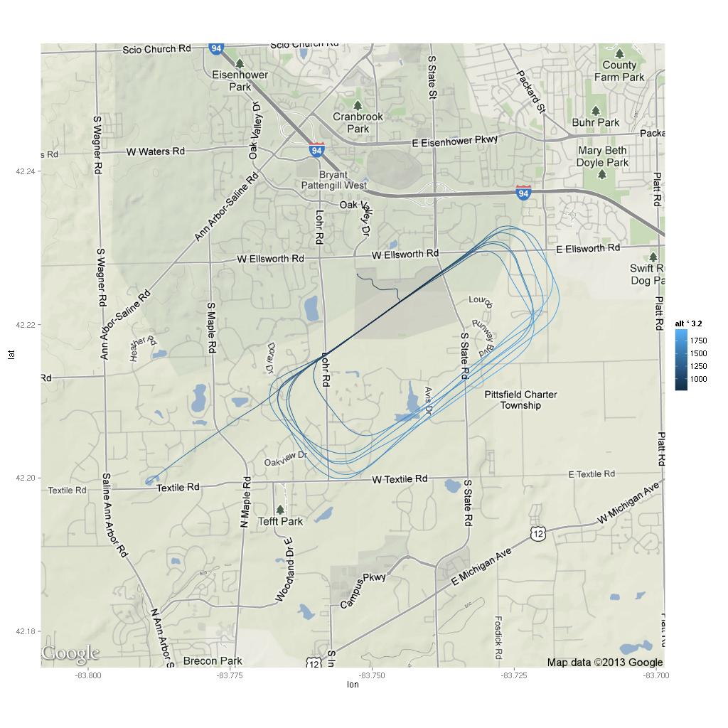
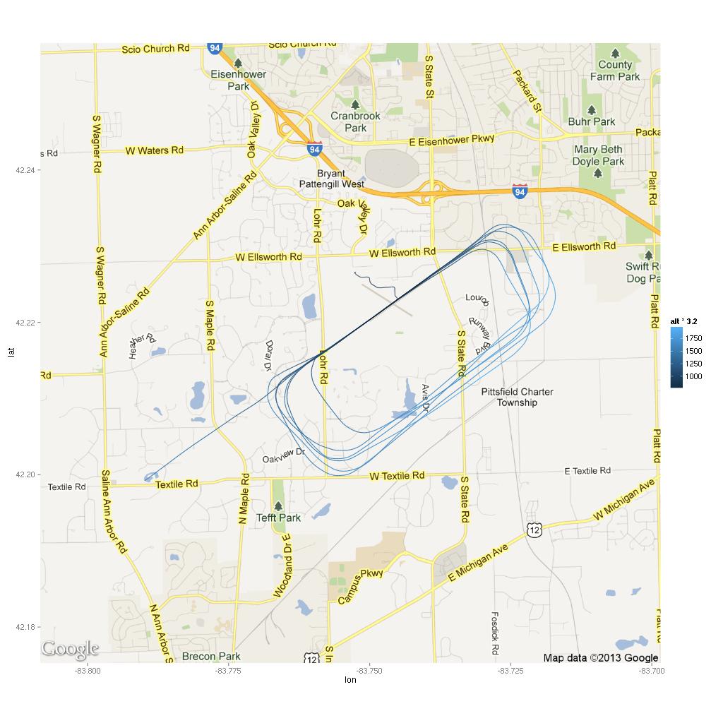
If you are wondering why the line doesn’t follow any roads… Roads? Where we’re going, we don’t need roads. (Hint: flying)

Here’s the entire script to get the plots:

#!/usr/bin/env Rscript

library(ggmap)

pts <- read.csv("gps.csv")

/* get the bounding box... left, bottom, right, top */
loc <- c(min(pts$lon), min(pts$lat), max(pts$lon), max(pts$lat))

for (type in c("roadmap","hybrid","terrain")) {
	print(type)
	map <- get_map(location=loc, zoom=13, maptype=type)
	p <- ggmap(map) + geom_path(aes(x=lon, y=lat, color=alt*3.2), data=pts)

	jpeg(paste(type, "-preview.jpg", sep=""), width=600, height=600)
	print(p)
	dev.off()

	jpeg(paste(type, ".jpg", sep=""), width=1024, height=1024)
	print(p)
	dev.off()
}

P.S. If you are going to use any of the maps for anything, you better read the terms of service.